how lossless audio compression works
nicholas chen · january 15, 2026 · 10 min read
with the rise of high-speed internet and cheap storage, lossless audio has moved from a niche audiophile obsession to a mainstream feature on platforms like apple music and tidal. but what is it, exactly? and can you even hear the difference?
what is lossless audio?
lossless audio refers to any audio format that preserves all of the data from the original source—usually a cd or a studio master. unlike lossy formats (like mp3 or aac), lossless compression doesn't throw away any information to save space. if you take a lossless file, decompress it, and compare it bit-for-bit to the original, they will be identical.
lossless vs lossy
lossy formats like mp3 work by using psychoacoustics to identify and remove parts of the sound that the human ear is less likely to hear. for example, if there's a very loud sound at one frequency and a much quieter sound at a nearby frequency, the mp3 encoder might just delete the quiet sound because your brain would "mask" it anyway.
lossless formats, on the other hand, don't care about what you can or can't hear. they treat the audio signal as a pure mathematical sequence and use advanced algorithms (like flac's linear prediction) to pack that data more efficiently without losing a single bit.
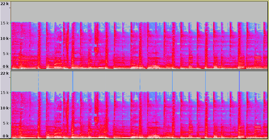
Lossiness: 55% · levels: 21 · kernel: 17 · Frequency: 0 – 3.9 kHz
common formats
there are several common lossless formats you'll encounter, each with its own pros and cons:
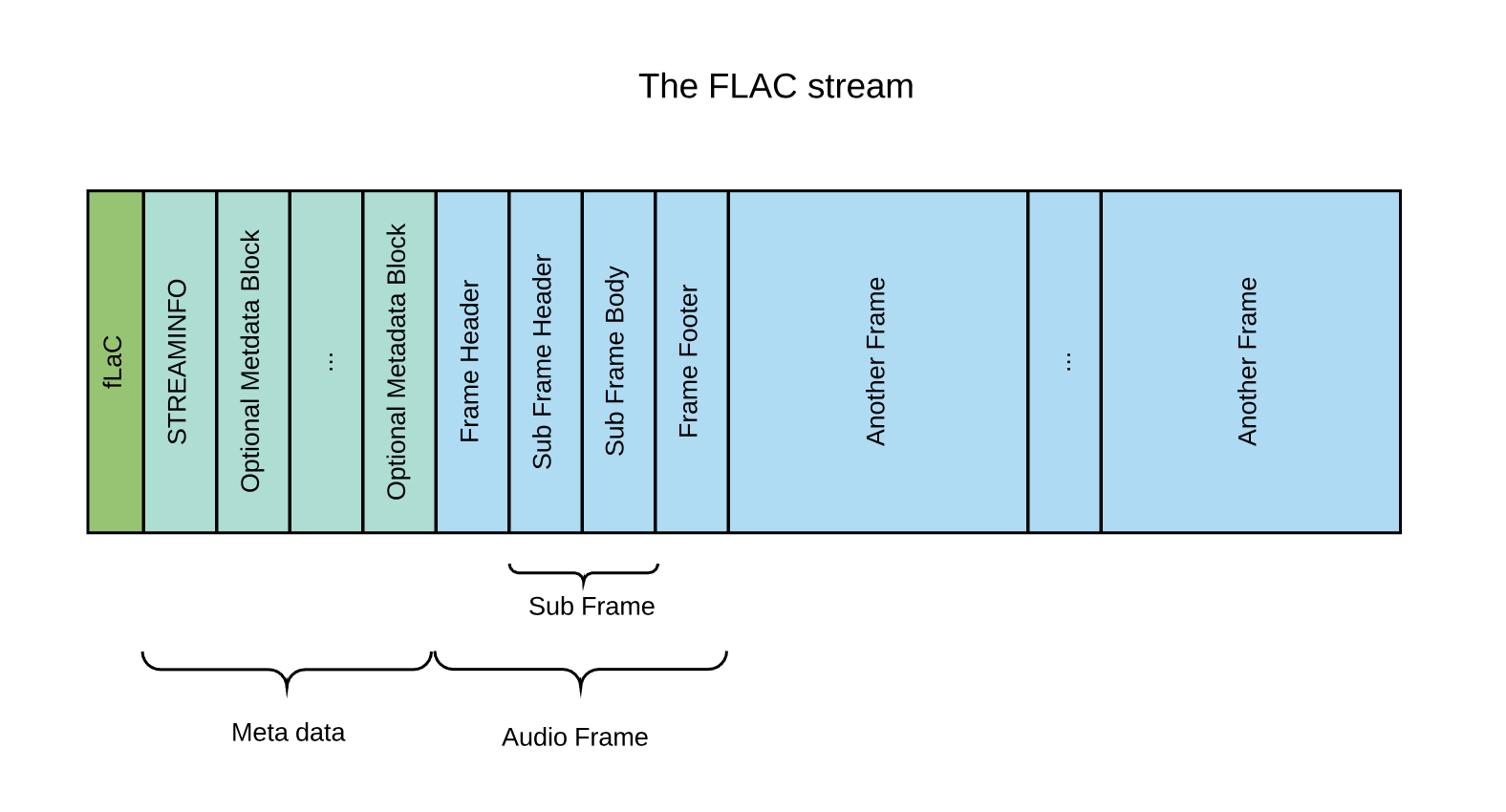
what is FLAC?
FLAC (free lossless audio codec) is the gold standard for lossless audio. it's open-source, widely supported, and offers excellent compression ratios (typically 50-60% of the original size). it also has great metadata support and is widely used for archiving music collections.
ALAC (apple lossless audio codec)
ALAC is apple's equivalent to flac. it's used by apple music and is the native lossless format for ios and macos devices. while it's now open-source, it's still primarily used within the apple ecosystem.
WAV / AIFF
these are uncompressed formats. they are literally just the raw pulse-code modulation (pcm) data. they don't use any compression at all, so they are perfectly lossless but take up about twice as much space as a flac or alac file.
mp3: under the hood
mp3 compression is fascinatingly complex. it uses a combination of subband coding, huffman coding, and a mdct (modified discrete cosine transform) to break the audio into small chunks and compress them. the result is a file that's roughly 10% of the original size but still sounds "good enough" for most people in most situations.
why does it matter?
for most casual listeners on bluetooth headphones, lossless audio won't make a difference because bluetooth itself uses lossy compression to transmit sound. however, if you have a high-quality wired setup (a good dac/amp and decent headphones), you might notice a wider "soundstage" and more clarity in complex passages of music.
let's be honest: for 99% of listening, a high-bitrate (320kbps) mp3 is indistinguishable from lossless. the real value of lossless is for archiving (having a perfect copy you can always transcode later) and for the peace of mind of knowing you're hearing exactly what the artist intended.
Note: It’s really hard to tell the difference for most people.
how is lossless audio compressed?
lossless compression works by finding patterns in the data and representing them more efficiently. the most common technique used in audio is linear prediction.
a deeper look into linear prediction
In digital audio, we have a sequence of samples: . These are the amplitudes of the sound wave at specific points in time.
Audio isn't random noise. If a sample is at a certain level, the next sample is likely to be very close to it. Linear prediction uses this fact to 'guess' the next sample based on previous ones.
The prediction is a weighted sum of previous samples: where are the predictor coefficients and is the 'order' of the predictor (how many previous samples we look at).
// Same example: p=3, coefficients a1=1.5, a2=-0.7, a3=0.2
const a = [1.5, -0.7, 0.2];
const prev = [100, 90, 80];  // x[n-1], x[n-2], x[n-3]

let pred = 0;
for (let k = 0; k < a.length; k++) pred += a[k] * prev[k];
// pred = 1.5*100 + (-0.7)*90 + 0.2*80 = 103

const xActual = 105;
const residual = xActual - pred;  // e[n] = 105 - 103 = 2
// Store residual (small) instead of 105 (large) → compression.
how do we find the best coefficients?
the encoder's job is to find the coefficients \( a_k \) that minimize the average size of the residuals. this is usually done using the levinson-durbin recursion or by solving the yule-walker equations.
We want to minimize the mean squared error:
by finding the 'best fit' line for the audio waveform in each small block of time, we can make the residuals as small as possible, which means we can represent them with fewer bits.
The Predictor Order ()
Higher orders of allow for more accurate predictions but require more computation. FLAC typically uses orders between 1 and 32. Simple signals like silence or pure sine waves only need low orders, while complex music might benefit from higher ones.
the key point
We aren't throwing away any data. The original sample is just . As long as we store the coefficients and the residuals, we can perfectly reconstruct the original signal.
what is 'n'?
'n' is the index of the current sample. In a standard CD-quality file, there are 44,100 samples per second. So goes from 0 up to 44,100 for each second of audio.
residuals: the 'leftovers'
The residual is the difference between what we predicted and what actually happened. Because our predictions are usually quite good, most residuals are very small numbers (close to zero).
storing small numbers takes fewer bits than storing large numbers. instead of using a full 16 bits for every sample, we might only need 2 or 3 bits for the residual of a well-predicted sample.
The residuals follow a Laplace distribution (centered at zero). We use entropy coding (like Rice coding) to assign shorter bit-sequences to the most common (smaller) residuals.
This is how we get a smaller file size while still guaranteeing that every bit can be restored during playback.
reconstructing the sound
During playback, your computer reads the coefficients and the sequence of residuals from the file. It then runs the same prediction formula and adds the residual back to get the exact original sample.
// Decoder: prediction + residual → original sample
const pred = 103;   // from same coefficients + previous samples
const residual = 2; // stored in the bitstream
const xReconstructed = pred + residual;  // 103 + 2 = 105 ✓
Rice Coding: Packing the Residuals
rice coding is a form of entropy coding that's particularly efficient for data following a laplace distribution (like audio residuals). it's a way to turn those small numbers into the shortest possible sequence of bits.
Rice coding uses a parameter . We split each number into two parts: a quotient and a remainder. The remainder is stored in binary, and the quotient is stored in unary.
For example, if we have a residual and we use :
The quotient (1) in unary is '01'. The remainder (2) in binary is '10'. So 6 is stored as '0110'.
Here's a comparison of how different residuals are stored with :
| residual (e) | standard binary (4-bit) | Rice code (k=2) |
|---|---|---|
| 0 | 0000 | 0 (1 bit) |
| 1 | 0001 | 010 (3 bits) |
| 2 | 0010 | 011 (3 bits) |
| 4 | 0100 | 10100 (5 bits) |
By choosing the optimal for each block of audio, FLAC can ensure that the residuals take up the absolute minimum amount of space possible.